Our Research Projects
I. Simple Interval Calculation (SIC)
Simple Interval Calculation (SIC) is a method of linear modeling
y = Xa + errors
that gives the result of prediction directly in the interval form. The
SIC also approach provides wide possibilities for the Object Status Classification,
i.e. leverage-type classification of relative importance of the calibration
and test sets samples with respect to a model.
Click the icon
 to open a PowerPoint file (= 870 kB) "Simple Interval Calculation (SIC) - Theory and
Applications", presented at the
Second Winter School on Chemometrics (WSC-2),
Barnaul, Russia, 2003.
to open a PowerPoint file (= 870 kB) "Simple Interval Calculation (SIC) - Theory and
Applications", presented at the
Second Winter School on Chemometrics (WSC-2),
Barnaul, Russia, 2003. |
Click
here
to ask for the file by e-mail |
The SIC approach is based on the single assumption that all errors are
limited (sampling errors, measurement errors, modelling errors), which would
appear to be reasonable in many practical applications. For prediction
modelling, this leads to results that are in a convenient interval form. The
SIC approach assesses the uncertainty of predicted values in such a way that
each point of the resulting interval has equal 'possibility'. The
SIC-interval is in contrast to the traditional confidence interval
estimators, which are based upon theoretical error distributional model
assumptions, which rarely hold for practical data analysis of technological
and natural systems. No probabilistic measure is introduced on the error
domain, therefore one does not have to evaluate the likelihood of the values
within the resulting prediction interval.
The finiteness of the error helps to construct the Region of Possible
Values (RPV) (Fig. I.1), a limited region in the parameter space that
includes all possible parameter values that satisfy the data set & model
under consideration.
Fig.I.1: Illustration of RPV in model parameter space.
The initial data set contains 24 objects but only 12
were necessary to form the RPV.
The SIC-approach does not use an(y) objective function (e.g. sum of
squares) for the parameter estimate search. In conventional regression
analysis these estimates are the values of unknown parameters, which agree
with the experimental data in the best way. In the SIC method any model
parameter value that does not contradict experimental data, i.e. lies inside
or on the border of RPV, is accepted as a feasible estimate.
The RPV concept provides wide possibilities for selection the samples from
calibration set that are of the most importance for model construction. This
is because the RPV is formed not by all objects from the calibration set,
but only by so-called boundary objects. Therefore, if we exclude all
objects from the calibration set except boundary ones, the RPV will not
change.
The position of a new objects (e.g. test set objects, or new X-data alone)
in relation to the RPV helps to understand the object
similarities/dissimilarities in comparison with those from the calibration
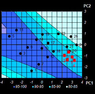
set. The object status map (see Fig. I.2), or so called the SIC
influence plot, can be constructed for any dimensionality of initial data
set [X, y] and any number of estimated model
parameters.
Fig. I.2: The example of Object Status map for real world data.
Samples С1-С11 ( )
are the calibration objects.
)
are the calibration objects.
Samples T1-T4 ( ) are
the test objects.
) are
the test objects.
Samples C2, C1, C6, and C11 are the boundary objects.
Sample T1 is an insider, sample T2 is an outsider
Sample T3 is an absolute outsider. Sample T4 is an outlier.
SIC returns an object status classification which divides the SIC-
residual vs. SIC - leverage plane into three categories: 'insiders'
(new objects very similar to the calibration set) and 'outsiders'
(all other objects in the rest of this plane. It is possible to establish a
further distinction between 'absolute outsiders' and more extreme 'outliers'.
Description of the SIC-method and the Object Status Classification
approach is published in --
O. Ye. Rodionova, K. H. Esbensen, and A.L. Pomerantsev,
"Application of SIC (Simple Interval Calculation) for object
status classification and outlier detection - comparison with PLS/PCR",
J. Chemometrics, 18 , 402-413 ( 2004)
DOI:10.1002/cem.885 |
Click
here
to ask for the file by e-mail |
No doubt that multivariate problems where data matrix is rank-
deficient are of great practical interest. To apply SIC-method to such
kind of problems we join it with traditional projection methods (e.g.,
principal component analysis or partial least squares).
We consider that the criteria of quality of interval prediction used
in SIC-procedure allow to look at the old problems of multivariate data
analysis from a new point of view. These problems are optimum number of
PCs, outlier detection, missing data, and insignificant observations. The roots of the method are in the old ideas of
Kantorovich to apply the linear programming to the data analysis. The
calculation aspects of SIC-method are rather simple since they founded
on the well-designed Simplex algorithm.
Now the SIC method is implemented in MATLAB script-language. The
software is presented
here.
An examples of the SIC-method are published in --
A.L. Pomerantsev, O.Ye. Rodionova, "Hard and soft
methods for prediction of antioxidants' activity based on the DSC
measurements", Chemom. Intell. Lab.Syst.,
79 (1-2), 73-83
(2005)
DOI:110.1016/j.chemolab.2005.04.004 |
Click
here
to ask for the file by e-mail |
A.L. Pomerantsev, O.Ye. Rodionova, A. Höskuldsson,
"Process control and optimization with simple interval calculation method",
Chemom. Intell. Lab.Syst., 81 (2), 165-179 (2006)
DOI:10.1016/j.chemolab.2005.12.005 |
Click
here
to ask for the file by e-mail |
| A.L. Pomerantsev and O.Ye. Rodionova, "Prediction
of antioxidants activity using DSC measurements. A feasibility study",
In Aging of Polymers, Polymer Blends and Polymer Composites, 2,
Nova science Publishers, NY, 2002, pp. 19-29 (ISBN 1-59033-256-3). |
Click
here
to ask for the file by e-mail |
| O.Ye. Rodionova, A.L. Pomerantsev, "Principles of
Simple Interval Calculations" In: Progress In Chemometrics
Research, Ed.: A.L. Pomerantsev, 43-64, NovaScience Publishers,
NY, 2005, (ISBN: 1-59454-257-0) |
Click
here
to ask for the file by e-mail |
| A.L. Pomerantsev and O.Ye. Rodionova,
"Multivariate Statistical Process Control and Optimization",
Ibid, 209-227 |
Click
here
to ask for the file by e-mail |
|

|

|
II. Nonlinear Regression
(NLR)
The main purpose of non-linear regression is to fit
data with a non-linear model, to predict response for predictor values that are
far from the observed ones, to estimate the uncertainties in prediction.
| Click the icon
to open a PowerPoint file (=1290 kB) "“Introduction to
non-linear regression analysis" (in Russian), presented at
the
Second Winter School on Chemometrics (WSC-2),
Barnaul, Russia, 2003. |
Click
here
to ask for the file by e-mail |
These ideas were implemented in the software
FITTER, a new
Excel Add-In.
Consider example of rubber aging prediction. Data of
accelerated aging tests, performed at temperatures: T=140C, 125C and 110C, are
presented in Fig II.1.
Fig II.1: Experimental data (left Y- and bottom X-axes)
and predicted kinetics (right Y- and top X-axes)
The response ELB is the 'Elongation at break' property that is
measured in accordance with ASTM D412-87. The data are fitted with the first
order kinetics, which rate constant k depends on temperature by the
Arrhenius law:
ELB=ELB1+(ELB0-ELB1)*exp(-k*t),
k=k0*exp[-E/(RT)],
where ELB0, ELB1, k0,
and E are unknown parameters. Prediction is performed at normal
temperature 20oC and the left (bottom) limits of confidence intervals are
obtained. This example is presented in:
E.V. Bystritskaya, O.Ye. Rodionova, and A.L.
Pomerantsev "Evolutionary Design of Experiment for Accelerated
Aging Tests", Polymer Testing, 19, 221-229, (1999)
DOI:10.1016/S0142-9418(98)00077-4 |
Click
here
to ask for the file by e-mail |
O. Y. Rodionova, A. L. Pomerantsev "Prediction of
Rubber Stability by Accelerated Aging Test Modeling", J Appl
Polym Sci, 95 (5) 1275-1284, (2005)
DOI:10.1002/app.21347 |
Click
here
to ask for the file by e-mail |
|
|
|
III. Statistics
Theoretical statistics is an area of our interests.
Making the forecast, it is essential to
find not only the point prediction value, but also to characterize the
uncertainty, which firstly depends on the extrapolation distance. Certainly, the
most convenient way is to present the result of prediction as a confidence
interval.
Fig III.1: Upper bounds of confidence intervals versus confidence
probability P for various methods: F, A, M, B,
L, S, and "exact" values T
We suggest a new method of confidence estimation for
NLR, where, unlike bootstrap, we simulate parameter estimates, not initial data.
The details are presented in
A.L. Pomerantsev "Confidence Intervals for Non-linear
Regression Extrapolation", Chemom. Intell. Lab. Syst, 49,
41-48, (1999)
DOI:10.1016/S0169-7439(99)00026-X |
Click
here
to ask for the file by e-mail |
The difference in the confidence intervals constructed
for a nonlinear model by various methods can be very great (see Fig. III.1), but in some cases
this difference could be negligible from the "engineering" point of
view. To explain this, we suggest a new coefficient of nonlinearity, which is
used for the decision-making about the method that can be utilized for a given
task. It is calculated by the Monte Carlo procedure and accounts for the model
structure as well as the experimental design features. More information about
the coefficient of nonlinearity is published in
These ideas were implemented in the software
FITTER, a new Excel Add-In.
|
|
|
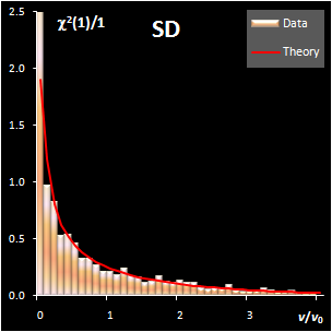
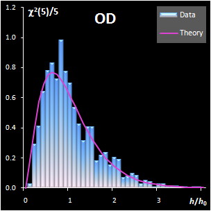
IV. SIMCA
In the projection methods (PCA, PLS) two distance
measures are of importance. They are the score distance (SD, a.k.a. leverage, h) and the orthogonal distance (OD, a.k.a. the
residual
variance, v). This research shows that both distance measures can be
modeled by the chi-squared distribution (Fig IV.1). Each model
includes a scaling factor that can be described by an explicit equation.
Moreover, the models depend on an unknown number of degrees of freedom (DoF),
which have to be estimated using a training data set. Such modeling is further
applied to classification within the SIMCA framework, and various acceptance
areas are built for a given significance level. .
 |
 |
|
Fig. IV.1: Example of the SD and OD distributions.
I=1440, A=6, Nh=5,
Nv=1 |
The SD and OD distributions are similar. Each of them
depends on a single unknown parameter, Nh and Nv
that are the effective DOFs. In our opinion, the estimation of DoF is a key
challenge in the projection modeling. In case of SD, DoF should be close to the
number of PCs used, i.e., Nh ≈A; and, in case of
OD, DoF is undoubtedly linked to the unknown rank of the data matrix, K=rank(X),
e.g. Nv ≈K–A. However, such evaluations
are valid only under an assumption that either data, or scores, are normally
distributed, which is always a dubious conjecture. Therefore, we believe that a
data-driven estimator of DoF, rather than a theory-driven one should be used.
The conventional method of moments is sensitive to outliers, therefore other
techniques have to be applied. The first approach is the robust estimation via
IQR estimator. The second way is the statistical simulation technique, such as
bootstrap and jackknife.
 |
 |
|
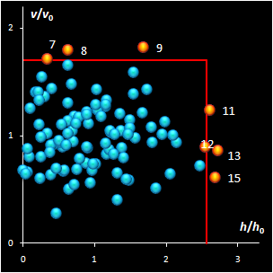
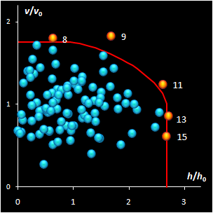
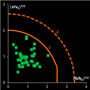
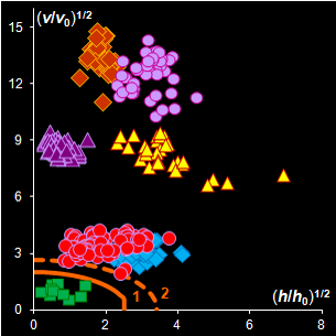
Fig. IV.2: SIMCA classification with the conventional
(left) and new (right) acceptance areas |
It is clear that any classification problem within the
projection approach should be solved with respect to a given significance level,
α,
i.e. the type I error. At the same time, the SD-OD, a.k.a. influence plot
is a valuable exploratory tool for the identification of the influential,
typical, extreme, and other interesting objects in data. In this plot different
acceptance areas can be constructed. They are the regions where a given share,
1–α, of the class members belongs to. Two of such areas are presented in
Fig. IV.2.
All of them are valid, i.e. they comply with the type
I error requirement, but not all of them are practical. Left panel shows the
conventional rectangle area, and the right panel represents the acceptance area,
which follows from the modified Wilson-Hilferty approximation of the chi-squared
distribution.
| Click the icon
to open a PowerPoint file (=3.3 MB) "Critical levels in
projection techniques ", presented at the
Six Winter Symposium on Chemometrics (WSC-6),
Kazan, Russia, 2008. |
Click
here
to ask for the file by e-mail |
A. Pomerantsev "Acceptance areas for multivariate
classification derived by projection methods", J. Chemometrics,
22, 601-609 (2008)
DOI: 10.1002/cem.1147 |
Click
here
to ask for the file by e-mail |
 |
 |
|
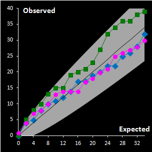
Fig. IV.3 : Extreme plots:
observed number of extreme objects vs. the expected number. Grey area
represents the 0.95 tolerance limits. |
For the construction of a reliable decision area in
the SIMCA method, it is necessary to analyze calibration data revealing the
objects of special types such as extremes and outliers. For this purpose a
thorough statistical analysis of the scores and orthogonal distances is
necessary. The distance values should be considered as any data acquired in the
experiment, and their distributions are estimated by a data driven method, such
as a method of moments or similar. The scaled chi-squared distribution seems to
be the first candidate among the others in such an assessment. This provides the
possibility of constructing a two-level decision area, with the extreme and
outlier thresholds, both in case of regular dataset and in the presence of
outliers. We suggest application of classical PCA with further use of enhanced
robust estimators both for the scaling factor and for the number of degrees of
freedom. A special diagnostic tool called Extreme plot is proposed for the
analyses of calibration objects (see Fig IV.3). Extreme objects play an important role in data
analysis. These objects are a mandatory attribute of any data set. The advocated
Dual Data Driven PCA/SIMCA (DD-SIMCA) approach has demonstrated a proper
performance in the analysis of simulated and real world data for both regular
and contaminated cases. DD-SIMCA has also been compared to ROBPCA, which is a
fully robust method
| Click the icon
to open a PowerPoint file (=3.2 MB) "Dual data driven SIMCA as a
one-class classifier", presented at the Nineth Winter Symposium on Chemometrics
(WSC-9),
Tomsk, Russia, 2014. |
Click
here
to ask for the file by e-mail |
A.L. Pomerantsev, O.Ye. Rodionova, "Concept and role of
extreme objects in PCA/SIMCA", J. Chemometrics,
28,
429–438 (2014)
DOI: 10.1002/cem.2506
|
Click
here
to ask for the file by e-mail |
Y.V. Zontov, O.Ye. Rodionova, S.V.
Kucheryavskiy, A.L. Pomerantsev, "DD-SIMCA – A MATLAB GUI tool
for data driven SIMCA approach", Chemom. Intell. Lab. Syst.
167, 23-28 (2017)
DOI:
10.1016/j.chemolab.2017.05.010 |
Click
here
to ask for the file by e-mail |
| Implementation of the Data-Driven SIMCA
method for MATLAB can
be downloaded from |
GitHub |
A novel method for theoretical calculation of the
type II (β) error in soft independent modeling by class analogy (SIMCA) is
proposed. It can be used to compare tentatively predicted and empirically
observed results of classification. Such an approach can better characterize
model quality, and thus improve its validation.
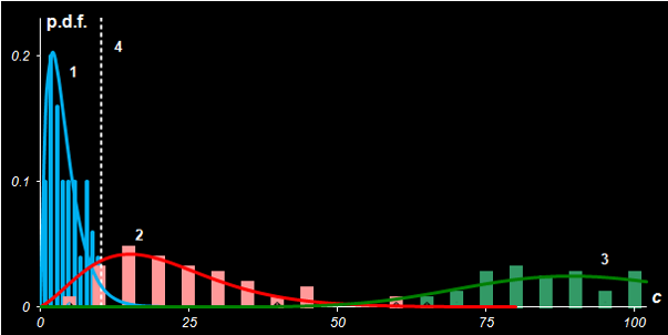
Fig IV.4: Fisher's Iris. Probability density distributions of
statistics c and c' in case
Versicolor (1) is the target class, while Virginica (2)
and Setosa (3) are the alternative classes.
Line 4 represents the critical cut-off value.
None of classification models are complete
without validation of the model quality, which is primarily associated
with the expected errors of misclassification. The type I error, α, is
the rate of false rejections (false alarm), i.e. the share of objects
from the target class that are misclassified as aliens. The type II
error β is the rate of false acceptances (miss), i.e. the share of
alien objects that are misclassified as the members of the target class.
When alternative classes are presented, the β-error can be calculated
for a given α-error as shown in Fig. IV.4. The α-error is equal to the
area under curve 1 to the right of line 4. The β-error is equal to the
area under curve 2 to the left of line 4. Moving critical level 4 we can
change the risks of wrong rejection (α) and wrong acceptance (β)
decisions.
A.L. Pomerantsev, O.Ye.
Rodionova, "On the type II error in SIMCA method", J.
Chemometrics, 28, 518-522 (2014)
DOI:
10.1002/cem.2610 |
Click
here
to ask for the file by e-mail |
 |
 |
|
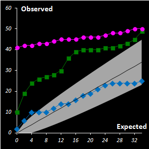
Fig. IV.5 : Amlodipine, producer A4 is used as the
target class. PCA model with two PCs.
Acceptance areas: regular at α= 0.01 (1);
extended at β = 0.005 (2). Left panel:
training set; right panel: test set. |
In counterfeit combating it is equally important to
recognize fakes and to avoid misclassification of genuine samples. This study
presents a general approach to the problem using a newly-developed method called
Data Driven Soft Independent Modeling of Class Analogy. In classification
modeling the possibility to collect representative data both for training and
validation is of great importance. In case no fakes are available, it is
proposed to compose the test set using the legitimate drug's analogues
manufactured by various producers. These analogues should have the identical API
and similar composition of excipients. The approach shows satisfactory results
both in revealing counterfeits and in accounting for the future variability of
the target class drugs. The presented in Fig. IV.5 a case study
demonstrates that theoretically predicted misclassification errors can be
successfully employed for the science-based risk assessment in drug
identification.
O.Ye. Rodionova, K.S. Balyklova,
A.V. Titova, A.L. Pomerantsev "Quantitative risk assessment in
classification of drugs with identical API content", J. Pharm.
Biomed. Anal. 98, 186-192 (2014)
DOI:
10.1016/j.jpba.2014.05.033 |
Click
here
to ask for the file by e-mail |
|
|
|
V. Successive
Bayesian Estimation
The successive Bayesian estimation (SBE) of regression
parameters is an effective technique applied in nonlinear regression analysis.
The main concept of SBE is to split the whole data set into several parts.
Afterwards, estimation of parameters is performed successively - fraction by
fraction - with Maximum Likelihood Method. It is important, that results
obtained on the previous step are used as a priori values (in the Bayesian form)
for the next part. During this procedure, the sequence of the parameter
estimates is produced and its last term is the ultimate estimate. Description of
SBE is published in
| G.A. Maksimova, A.L. Pomerantsev, "Successive Bayesian
Estimation of Regression Parameters", Zavod. Lab., 61,
432-435, (1995) |
|
It was shown that this technique is correct and it
gives the same values of estimates for linear regression as the traditional
OLS approach. Moreover, in that case, the result does not depend on the
order of the series. In non-linear regression case, the situation becomes
more difficult but we can pose that all these properties are asymptotically
the same.
| Click the icon
to open a PowerPoint file (=1890 kB) "Successive Bayesian estimation for linear and
non-linear modeling", presented at the Second Winter School on
Chemometrics (WSC-2),
Barnaul, Russia, 2003 ) |
Click
here
to ask for the file by e-mail |
This method is
used for obtaining kinetic information from spectral data without any pure
component spectra (Fig. V.1, left). With the help of real-world example, this approach is
compared with known methods of kinetic modeling (Fig V.1, right).
 |
 |
|
Fig. V.1: Successive estimates of kinetic
parameters (left panel) and
ultimate estimates with
various methods presented by the 0.95 confidence ellipses (right
panel) |
This example is
presented in
A.L. Pomerantsev "Successive Bayesian estimation
of reaction rate constants from spectral data", Chemom. Intell. Lab. Syst,
66 (2), 127-139 (2003)
DOI:10.1016/S0169-7439(03)00028-5 |
Click
here
to ask for the file by e-mail |
O.Ye Rodionova, A.L Pomerantsev "On One Method of
Parameter Estimation in Chemical Kinetics Using Spectra with Unknown
Spectral Components", Kinetics and Catalysis, 45
(4): 455-466, (2004)
DOI: 10.1023/B:KICA.0000038071.51067.d5 |
Click
here
to ask for the file by e-mail |
|
|
|
VI. Fitter Add-In
FITTER is an Add-In procedure for Excel. If you are under Excel you can
open FITTER as any add-in file using Tools/Add-Ins menu command. It
will add the new menu item Fitter into Tools menu. Clicking it, the main
Fitter dialog for starting FITTER is activated.
Fig. VI.1: Main Fitter dialog
FITTER is a powerful instrument of statistical analysis. Using it you may
solve multivariate nonlinear regression problems. Much of the power of
FITTER comes from its ability to estimate parameter values of complicated
user-defined functions that may be entered in ordinary algebraic notation as
a set of explicit, implicit and ordinary differential equations. FITTER uses
the unique procedure for analytic calculation of derivatives and special
optimization algorithm which provides the high accuracy even for
significantly nonlinear models. All complicated calculations are performed
in the special DLL library created using C++ compiler, which provides high
speed processing. FITTER allows to include prior knowledge about parameters
and accuracy of measurement in addition to experimental data. Using Bayesian
estimation, you can process both unlimited arrays of single-response data,
and data referring to different responses.
| Click the icon
to open a PowerPoint file (=1290 kB) "Non-linear Regression Analysis with Fitter
Software Application", presented at the First Winter School on
Chemometrics (WSC-1),
Kostroma,
Russia, 2002. |
Click
here
to ask for the file by e-mail |
With the help of FITTER you can obtain a lot of additional statistical
information concerning the input data and the quality of fitting. Parameter
estimates, variances, covariance matrix, correlation matrix and F-matrix;
the starting and final values of the sum of squares and objective function,
error variance, and spread in eigenvalues of the Hessian matrix; error
variance for each observation point calculated by fit and by population.
Moreover, there are hypotheses testing for: Student's test for outliers,
test of series for residual correlation, Bartlett's test for
homoscedastisity, Fisher's test for goodness of fit. Also, you can calculate
confidence intervals for each observation point by linearization method or
with the help of modified bootstrap technique. Detailed description of
Fitter application is presented in
FITTER takes all information from open Excel workbook. Information should
be placed directly on a worksheets (Data and Parameters) or written in a
text box (Model). All results are also output as tables on the worksheets.
In purpose to explain what information you want to use, you need to register
it with the help of FITTER wizards. There are DATA, MODEL and BAYES
registration wizards. While working with different FITTER wizards you only
register the required information, change options and look through process
of registration. You may change data only on the worksheets but not inside
the wizards. Since your information (Data, Model, ...) has been registered
it is kept in memory till you replace it by another registration.
An example of Fitter application to the diffusion problems solution is
published in
A. L. Pomerantsev "Phenomenological modeling of
anomalous diffusion in polymers", J Appl Polym Sci, 96(4)
1102 - 1114, (2005)
DOI:10.1002/app.21540 |
Click
here
to ask for the file by e-mail |
Estimation of the parameters of the Arrhenius equation often leads to
multicollinearity, or, in other words, a degenerate set of equations in the
least-squares procedure. This circumstance makes it difficult to estimate
the unknown parameters. Simple expedients for model modification are
considered that reduce multicollinearity.
O. E. Rodionova, A. L. Pomerantsev "Estimating the
Parameters of the Arrhenius Equation", Kinetics and Catalysis,
46, 305–308, (2005).
DOI: 10.1007/s10975-005-0077-9 |
Click
here
to ask for the file by e-mail |
Click here to
know more about Fitter software.
|
|
|
VII. Counterfeit Drug
Detection
The problem of counterfeit drugs is important all
over the world. For the first time the World Health Organization (WHO)
obtained information about forgeries in 1982. At that time counterfeit drugs
were mainly found in the developing countries. The definition for “counterfeit
drug” by WHO is as follows: “A counterfeit medicine is one which is
deliberately and fraudulently mislabeled with respect to identity and/or
source. Counterfeiting can apply to both branded and generic products and
counterfeit products may include products with the correct ingredients or
with the wrong ingredients, without active ingredients, with insufficient
active ingredient or with fake packaging”
Nowadays, there are “high quality” counterfeit
drugs that are very difficult to detect. It is worth mentioning that fake
drugs include dietary supplements too. In such medicine non-declared
substances such as hormones, ephedrine, etc., may be found. According to WHO
information the spread of counterfeit drugs in different countries are as
follows: 70% of turnover is in developing countries and 30% is in
market-economy countries. The distribution of fake drugs with respect to
different therapeutic groups is as follows: (1) antimicrobial drugs 28%; (2)
hormone-containing drugs 22% (including 10% of steroids); (3) antihistamine
medicines 17%; (4) vasodilators 7%; (5) drugs used for treatment of sexual
disorders 5%; (6) anticonvulsants 2%; (7) others 19%. Visual control,
disintegration tests or simple color reaction tests reveal only very rough
forgeries. More complicated chemical methods are also used but all
these methods try to prove or disprove the content and concentration of an
active ingredient. But the main goal is to discriminate genuine and
counterfeit drug, even in cases where the counterfeit drug contains the
sufficient concentration of active ingredient and as a result to answer the
question: “Does given drug correspond to the original as it is marked on
the package?”
Express-methods for detection of counterfeit drugs
are of vital necessity. In many cases dosage forms contain not only active
substances but also excipients. The exact content of excipients could differ
for the genuine and fake drugs. It is proposed to apply near infra-red (NIR)
spectroscopy that could be used both for identification of
pharmaceutical substances and dosage forms independently of contents of an
active ingredient. NIR also could give information about the excipients in a
pharmaceutical preparation and thereby be able to detect counterfeit drugs
even with proper active substance. A feasibility study has been published in
O.Ye. Rodionova, L.P. Houmøller, A.L. Pomerantsev, P.
Geladi, J. Burger, V.L. Dorofeyev, A.P. Arzamastsev "NIR
spectrometry for counterfeit drug detection", Anal. Chim. Acta,
549, 151-158 (2005)
DOI:10.1016/j.aca.2005.06.018 |
Click
here
to ask for the file by e-mail |
Two grades of tablets (antispasmodic drug,
uncoated tablets, 40 mg) are investigated. Ten genuine tablets, subset N1,
and 10 forgeries, subset N2 were measured using the InAs detector. After
that one tablet from set N1 was cut in half and a spectrum of the interior
of a cut tablet was measured; this was named N1Cut. The same procedure was
done for one tablet from set N2. As a result, in total 22 spectra were
obtained. These spectra were pre-treated by MSC and are shown in Fig.
VII.1.
Fig VII.1: MSC pre-treated spectra . Blue lines (N1) are 11 genuine tablets
spectra
and red lines (N2) are 11 counterfeit tablets spectra.
The data are subjected to a principal component
analysis. Taking into account two principal components (PCs) we come to the
following results (Fig. VII.2, left). Two manifest clusters in the PC1–PC2
plane are seen. Thus, the subsets N1 and N2 may easily be discriminated. The
object variance in subset N2 (counterfeit drug) is significantly greater
than the variance between objects in subset N1 (genuine tablets). This may
be explained by better manufacturing control for genuine tablets. Spectra
for the cut tablets are similar to the spectra of the whole tablets (compare open
dots).
 |
 |
|
Fig. VII.2: PCA scores plot (left panel) and SIMCA
plot (right
panel). Blue dots represent genuine tablets (N1)
and red squares represent counterfeit tablets (N2). Open dots
and squares show cut tablets. |
SIMCA method is applied to discriminate class N1
(genuine tablets) from any other counterfeit tablets .The “membership
plot” that presents the distance to model si
versus leverage hi is shown in Fig. 10, right panel.
The limits are shown as white lines: horizontal for the distance to model
and vertical for the leverage. It may be easily seen that the N1Cut object has a
low leverage, but its distance to the model is greater than the limit
though it lies not far from the model. Samples from set N2 are very far from
the model and undoubtedly can be classified as non-members of this
class.
In general, there is one class of genuine drug
samples and there may be plenty of forgeries of different degrees of
similarity. Due to the production quality demands in the large
pharmaceutical plants, the differences between the genuine items are rather
small. Nevertheless, we consider this investigation as a feasibility study
that yields promising results. For more trustworthy modeling it is necessary
to collect a representative set of genuine samples of the drug produced at
different times, with different shelf life, etc. On the other hand, the
diversity inside the counterfeit samples is essentially large. Sometimes the
difference between the genuine and counterfeit drugs could be seen visually
in the NIR spectra, but in other situations the answer is not so evident. To
claim that a sample is a forgery, it is not necessary to compare the
concentrations of active ingredients. All that is needed is to check whether
a given sample is identical to the genuine drug or not. The above analysis
shows that the NIR approach together with PCA has the good prospects and may
efficiently substitute wet chemistry.
This a common opinion that the NIR spectroscopy is
a low sensitive method. However, being combined with a proper chemometric
analysis, this method demonstrates excellent results, which often are even
better (or compatible) than conventional "wet chemistry" approach. This study confirms this claim. The research is based on the case study of injection of Dexamethasone, which is a glucocorticosteroid remedy. The manufacturer
detected a batch of forgery medicine in the pharmaceutical market by
revealing the lack of several printing marks, which are hidden in the
package for security reasons. At the same time the standard pharmacopoeia
tests (GC-MS) held at the manufacturer facility did not confirm the counterfeiting
since the quality and quantity of the active substance was within the
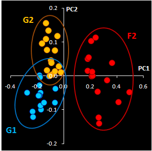
standards. Later the suspicious drug (labeled F2) and genuine samples
(labeled G1 and G2) with identical
batch numbers (G2 and F2) were subjected to the NIR based analysis.
 |
 |
|
Fig. VII.3: Raw NIR spectra (left panel).
30 genuine samples G1 & G2 (blue) and 15 fakes F2 (red).
PCA
plot (right
panel). Blue and yellow dots represent G1 & G2, red ones stand for F2. |
NIR spectra (Fig VII.3, left) were
obtained through the closed ampoules. PCA (Fig VII.3, right)
confirmed that genuine series G1 and G2 are very similar, but
suspicious sample F2 differs.
To compare the chemometrics based solution with
the conventional analytical methods the ampoules were opened and the drug
was subjected to the GC-MS, HPLC-DAD-MS, and CE-UV techniques. HPLC-DAD
chromatograms of the suspicious F2 and the genuine (G2 and G1) samples are shown
in Fig. VII.4.
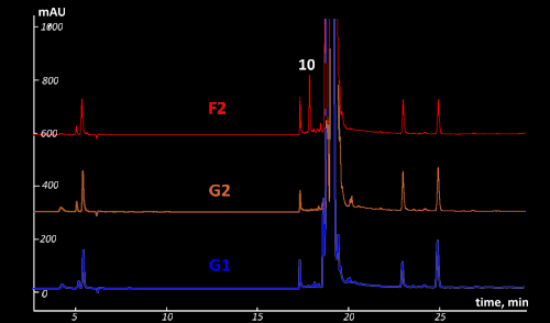
Fig VII.4: Comparison of the HPLC-DAD chromatograms of the fake (F2) and
original (G2 and G1) samples. UV detection at 254 nm.
Mind peak (10) for suspicious sample F2. This peak
is absented for genuine samples G1 & G2
The results of the NIR tests have been completely
confirmed by the intensive chemical studies. Samples from batches G1 and G2
similar in their impurity composition but differ in the quantity of the
impurities. Difference in impurity composition reflects in NIR spectra and
helps easily to disclosure the counterfeited samples.
| Click the icon
to open a PowerPoint presentation (=1.1 MB) "Another proof
that chemometrics is usable: NIR confirmed by HPLC-DAD-MS and CE-UV ", presented at
the Seventh Winter Symposium on
Chemometrics (WSC-7),
St Petersburg, Russia, 2010 ) |
Click
here
to ask for the file by e-mail |
O.Ye. Rodionova, A.L. Pomerantsev, L. Houmuller,
A.V.Shpak, O.A. Shpigun " Noninvasive detection of counterfeited
ampoules of dexamethasone using NIR with confirmation by HPLC-DAD-MS and
CE-UV methods " Anal Bioanal Chem 397, 1927–1935 (2010)
DOI: 10.1007/s00216-010-3711-y |
Click
here
to ask for the file by e-mail |
There is no simple solution to the problem of
counterfeit drug detection. The so-called 'high quality fakes' with proper
composition are the most difficult to reveal. The methods based only on
quantitative determination of active ingredients are sometimes insufficient.
A more general approach is to consider a remedy as a whole object, taking
into account a complex composition of active ingredients, excipients, as
well as manufacturing conditions, such as degree of drying, etc. The
application of NIR measurements combined with chemometric data processing is
an effective method but its superficial application simplicity may lead to
wrong conclusions that undermine confidence in the technique. The main
drawback of the NIR-based approach is the necessity to apply
multivariate/chemometric data analysis in order to extract useful
information from the acquired spectra.
 |
 |
|
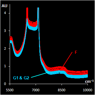
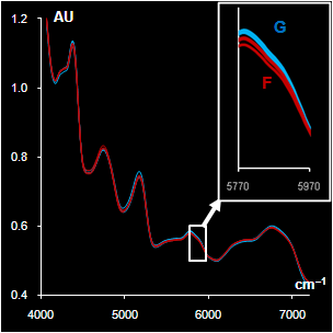
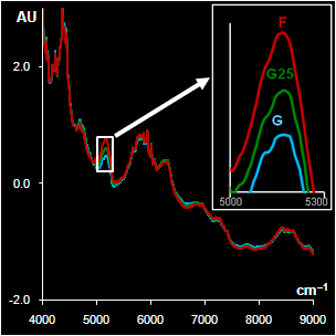
Fig. VII.5: Spectra after
pre-processing: blue (green) lines G are genuine samples, red
lines F are counterfeit samples
Left. Sildenafil. The whole spectra and the range selected by a
program
Right Metronidazole. The whole spectra and the range with high water
influence |
We've published an overview of the experience
of different research groups in NIR drug detection and highlights the main
issues that should be taken into account. The common problems to be dealt
with are the following:
(1) each medical product should be carefully tested
for a batch-to-batch variability;
(2) the selection of a specific spectral
region and the data pre-processing method should be done for each type of
medicine individually;
(3) it is crucial to recognize counterfeits as well
as to avoid misclassification of the genuine samples.
The real-world
examples presented in the paper illustrate these statements.
O.Ye. Rodionova, A.L. Pomerantsev,"NIR
based approach to counterfeit-drug detection"
Trends Anal. Chem., 29 (8),
781-938 (2010)
DOI: 10.1016/j.trac.2010.05.004 |
Click
here
to ask for the file by e-mail |
|
|
|
VIII. PAT & QbD
Process Analytical Technology
(PAT) and Quality by
Design (QbD) are the novel approaches for designing, analyzing, and controlling
manufacturing through timely measurements (i.e., during processing) of critical
quality and performance attributes of raw and in-process materials and
processes, with the goal of ensuring final product quality. Several studies in
this area have been performed in the group.
Methods of process control and optimization are
presented and illustrated with a real world example. We
considered a multi-stage technological process that is represented by 25 process
variables and one output variable, y, which is the final quality of the end-product.
The production cycle (see
Fig.
VIII.1) is divided
into seven stages numbered by the Roman numerals. Each stage may be described by
the input, current, and further variables. Variables used in all previous stages
are fixed input variables, current variables are the controlled ones, and the
variables that characterize the following production stages are out of scope at
the moment. Moving along the process, variables change their roles.
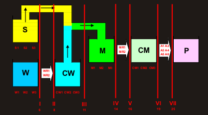
Fig. VIII.1: Production cycle
The optimization methods
are based on the PLS block modeling as well as on the Simple
Interval Calculation methods of interval prediction and object status
classification. It is proposed to employ the series of expanding PLS/SIC models
in order to support the on-line process improvements. This method helps to
predict the effect of planned actions on the product quality, and thus enables
passive quality control. We have also considered an optimization approach that
proposes the correcting actions for the quality improvement in the course of
production. The latter is an active quality optimization, which takes into
account the actual history of the process. The advocate approach is allied to
the conventional method of multivariate statistical process control (MSPC) as it
also employs the historical process data as a basis for modeling. On the other
hand, the presented concept aims more at the process optimization than at the
process control. Therefore, it is proposed to call such an approach as
multivariate statistical process optimization (MSPO).
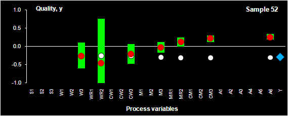
Fig. VIII.2: Process optimization. SIC intervals (green bars), PLS prediction
(red dots) for sample 52.
Blue rhombus shows the historical quality value, y, that was actually obtained
in the production.
White dots represent the PLS predictions for the control set.
| Click the icon
to open a PowerPoint file (=1MB) "Multivariate
Statistical Process Optimization ", presented at the Third Winter School on
Chemometrics (WSC-3),
PushGory , Russia, 2004 |
Click
here
to ask for the file by e-mail |
A.L. Pomerantsev, O.Ye. Rodionova, A. Höskuldsson,
"Process control and optimization with simple interval calculation method",
Chemom. Intell. Lab.Syst., 81 (2), 165-179 (2006)
DOI:10.1016/j.chemolab.2005.12.005 |
Click
here
to ask for the file by e-mail |
The possibility of routine testing of pharmaceutical
substances directly in warehouses is of great importance for manufactures,
especially taking into account the demands of PAT. The application of NIR
instruments with remote fiber optic probe makes these measurements simple and
rapid. On the other hand carrying out measurements through closed polyethylene
bags is a real challenge. To make the whole procedure reliable we propose the
special trichotomy classification procedure. The approach is illustrated by a
real-world example.
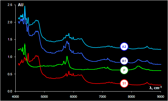
Fig. VIII.3: Spectrum S1 obtained from sample 1 without PE bag (substance), P
is a spectrum of PE bag,
A1 is a spectrum of sample 1 in PE bag, A2 is a spectrum of sample 2 in PE bag
The substance under investigation is Taurine, a
non-essential sulfur-containing amino acid. The NIR spectra were recorded with a
hand held diffuse reflectance fiber optic probe. The spectra were measured
through closed polyethylene (PE) bags in the 4000 – 10000 cm-1 region. The
explorative PCA of the dataset shows an essential difference between
the samples (Fig. VIII.3). More than 60 objects (out of 246) may be treated as doubtless
outliers. The source of such variations was found after comparing the spectra of
the substance in a bag, the spectra of unpacked substance (S1), and the spectra
of empty polyethylene bags (P).
Samples that are measured successfully (through a single PE layer) belong to
Class 1. Other samples that are not measured carefully (through the several PE
layer) are attributed to Class 2. Two corresponding SIMCA models participate in
the following routine testing procedure.
- If a sample belongs to Class 1 (Model 1), this is a sample of a
satisfactory quality (decision “accepted”);
- If a sample belongs to Class 2 (Model 2), measurement should be repeated
(no decision);
- If a sample does not belong to Class 2, such a sample is an alien
(decision “rejected”).
The flowchart of the routine testing is shown in Fig. VIII.4
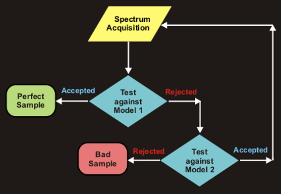
Fig. VIII.4: The flowchart of the sample routine testing
.Ye. Rodionova, Ya.V. Sokovikov, A.L. Pomerantsev "
Quality control of packed raw materials in pharmaceutical industry"
Anal. Chim. Acta , 642(1-2), 222-227 (2009)
DOI:
10.1016/j.aca.2008.08.004 |
Click
here
to ask for the file by e-mail |
This QbD research is aimed at optimization of a hybrid binder formulation that
includes water solution of sodium silicate (water glass) and polyisocyanate.
Optimization is performed with respect to twelve output quality characteristics.
Calibration modeling is done as a two-step NPCR procedure. At first, PCA is
applied to the X- block for variable reduction. Then nonlinear regression is
used to predict a particular quality characteristic as a function of score
vectors. The input variables reduction enables to choose an optimal binder
formulation that meets the predefined quality requirements.
 |
 |
|
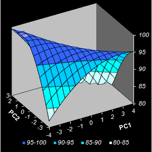
Fig. VIII.5: Conversion level predicted by NPCR.
Color intensity reflects the property value.
Contour map. Black dots are the calibration points, red squares are optimized test
points (Left);
3-D surface model (Right) . |
The study demonstrates the benefits of chemometric approach in application to
chemical engineering. The non-linear PCR solves a complex nonlinear multivariate
optimization problem employing a simple projection approach and graphical
representation of the models. The input variables' reduction gives an
opportunity to choose the optimal binder formulations visually without
complicated numerical procedures.
I.A. Starovoitova, V.G. Khozin, L.A. Abdrakhmanova,
O.Ye. Rodionova, A.L. Pomerantsev "Application of nonlinear PCR for
optimization of hybrid binder used in construction materials", Chemom.
Intell. Lab.Syst., 97 (1), 46-51 (2009)
DOI:
10.1016/j.chemolab.2008.07.008 |
Click
here
to ask for the file by e-mail |
A new method for prediction of the drug release
profiles during a running pellet coating process from in-line near infrared
(NIR) measurements has been developed. The NIR spectra were acquired during a
manufacturing process through an immersion probe. These spectra reflect the
coating thickness that is inherently connected with the drug release. Pellets
sampled at nine process time points from thirteen designed laboratory-scale
coating batches were subjected to the dissolution testing. In the case of the
pH-sensitive Acryl-EZE coating the drug release kinetics for the acidic medium
has a sigmoid form with a pronounced induction period that tends to grow along
with the coating thickness. In this work the autocatalytic model adopted from
the chemical kinetics has been successfully applied to describe the drug
release. A generalized interpretation of the kinetic constants in terms of the
process and product parameters has been suggested. A combination of the kinetic
model with the multivariate Partial Least Squares (PLS) regression enabled
prediction of the release profiles from the process NIR data. The method can be
used to monitor the final pellet quality in the course of a coating process
Fig. VIII.6: Research goal
A valuable theoretical result is the solution of the
“curve-to-curve” calibration problem and in the particular case considered here,
the prediction of the drug release profiles from NIR spectra. This method
differs from the conventional approach, where a curve is restored from the
individually calibrated and predicted points. The advocated approach extracts
new features as the parameters of a function approximating the drug release
profile. Such a function can be selected on a purely empirical basis, or derived
from the fundamental process knowledge. Additionally, successful approximation
results in a considerable data reduction. The main merit however is the ability
to predict the whole curve smoothly.
 |
 |
|
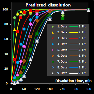
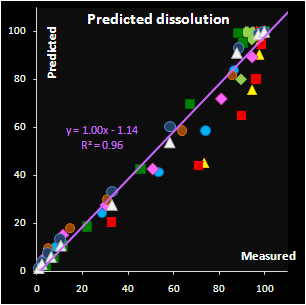
Fig. VII.7: Predicted API release curves |
It has been found that the autocatalytic model
perfectly fits the drug release kinetics of the pellets coated by a
pH-sensitive polymer. Moreover, two underlying kinetic constants have a
reasonable physical interpretation. The first parameter, m, is
responsible for the coating material grade and this parameter varies
neither within a batch nor between the similar batches. The second
parameter, k, is closely related to the coating thickness and this
dependence is individual for every batch. Subsequently, the
autocatalysis is a mechanical rather than a purely empirical model. A
preliminary explanation of the mechanism's nature has been suggested.
Click the icon
 to open presentation (=1.3 MB) "In-line prediction of drug
release profile for pH-sensitive coated pellets", 12- th
International Conference on Chemometrics in Analytical Chemistry
(CAC-2010), Antwerp, Belgium, 2010
to open presentation (=1.3 MB) "In-line prediction of drug
release profile for pH-sensitive coated pellets", 12- th
International Conference on Chemometrics in Analytical Chemistry
(CAC-2010), Antwerp, Belgium, 2010 |
Click
here
to ask for the file by e-mail |
IX. Chemometrics in Excel
Chemometrics is a very practical discipline. To learn
it one should not only understand the numerous chemometric methods, but also
adopt their practical application. This book can assist you in this difficult
task. It is aimed primarily at those who are interested in the analysis of
experimental data: chemists, physicists, biologists, and others. It can also
serve as an introduction for beginners who start learning about multivariate
data analysis.
 |
 |
|
Fig. IX.1: Russian & English editions of the
book |
| A.L. Pomerantsev, Chemometrics in Excel, Wiley, 336
pages, 2014 , ISBN: 978-1-118-60535-6 |
Click
here
to order the book |
| Померанцев А.Л. Хемометрика в Excel: учебное пособие,
Томск, Из-во ТПУ, 435 стр.,2014, ISBN 978-5-4387-0374-7 |
|
The conventional way of chemometrics training utilizes
either specialized programs (the Unscrambler, SIMCA, etc.), or the MatLab. We
suggest our own method that employs the abilities of the world’s most popular
program, Microsoft Excel®. However, the main chemometric algorithms, e.g.
projection methods (PCA, PLS) are difficult to implement using basic Excel
facilities. Therefore, we have developed a special supplement to the standard
Excel version called Chemometrics AddIn, which can be used to perform such
calculations. In this case all calculations are carried out in the open Excel
books. Moreover all regular Excel capacities can be applied for additional
calculations, graphical presentations, export and import of data and results,
customizing individual templates, etc. Excel 2007 gives additional incentive to
this idea as now very large arrays (1,048,576 rows by 16,384 columns) can be
input and processed directly in the worksheets. We have designed the core
functions for the PCA/PLS decompositions and ensured that calculations are
performed very quickly even for rather large data sets (200 samples by 4500
variables). These functions are programmed in C++ language and linked to Excel
as an Add-In tool named Chemometrics Add-in.
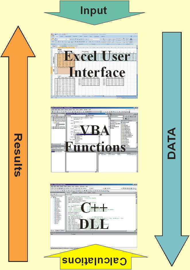
Fig IX.2: Software flow-chart
We designed "Chemometrics" as an Add-In
procedure for Excel. This add-in file is opened by a Tools/Add-Ins menu
command. After that, main projection functions can be applied as ordinary
user-defined functions in Excel.
-
All calculations are carried out in the open
Excel books.
-
All results are also output as tables on the
worksheets.
-
All calculations are made "on the
fly".
-
As soon as a user changes any cell in the
input data, output data are recalculated automatically (if
"automatic" option is switched on in a
Tools/Options/Calculation menu).
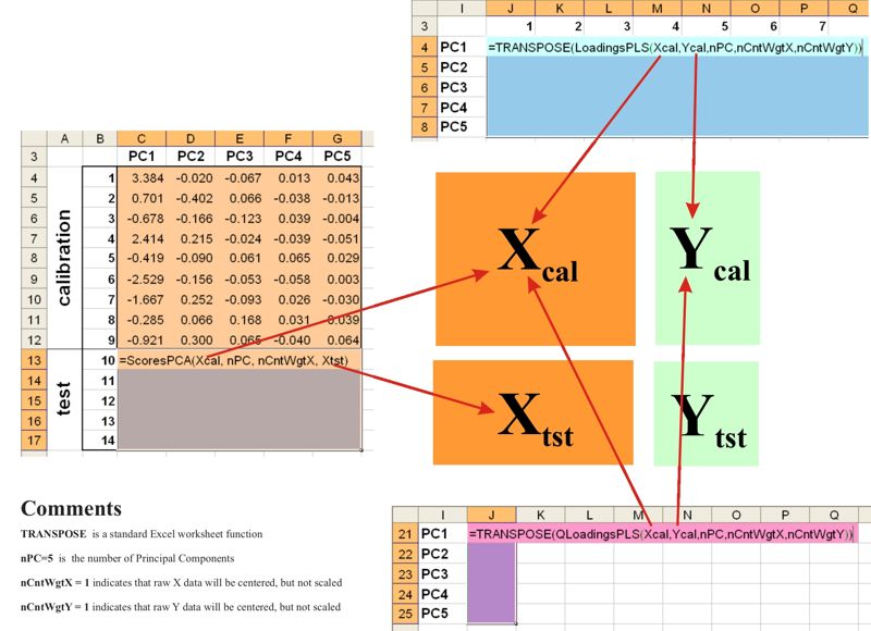
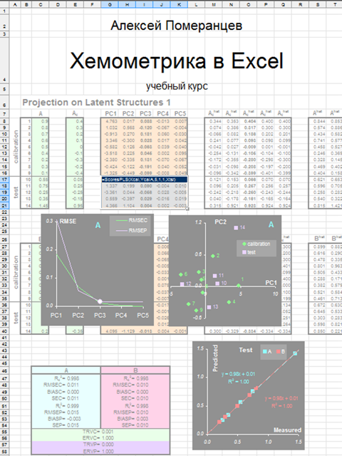
Fig IX.3: Common worksheet layout for application of Chemometrics Add-In
List of user-defined
functions
PCA Decomposition
-
ScoresPCA (X, PC, CentWeight, Xnew )
-
LoadingsPCA (X, PC, CentWeight )
PLS Decomposition
-
ScoresPLS (X, Y, PC, CentWeightX, CentWeightY
, Xnew)
-
UScoresPLS (X, Y, PC, CentWeightX, CentWeightY,
Xnew, Ynew )
-
LoadingsPLS (X, Y, PC, CentWeightX, CentWeightY )
-
WLoadingsPLS (X, Y, PC, CentWeightX, CentWeightY )
-
QLoadingsPLS (X, Y, PC, CentWeightX, CentWeightY )
PLS2 Decomposition
-
ScoresPLS2 (X, Y, PC, CentWeightX, CentWeightY
, Xnew)
-
UScoresPLS2 (X, Y, PC, CentWeightX, CentWeightY,
Xnew, Ynew )
-
LoadingsPLS2 (X, Y, PC, CentWeightX, CentWeightY )
-
WLoadingsPLS2 (X, Y, PC, CentWeightX, CentWeightY )
-
QLoadingsPLS2 (X, Y, PC, CentWeightX, CentWeightY )
| Click the icon
to open a PowerPoint file (=2335 kB) "Chemometric functions in Excel", presented at
the First
Symposium of South African Chemometrics Society (Stellenbosch
University, South Africa). |
Click
here
to ask for the file by e-mail |
Click
here
to
know more about Chemometrics Add-In.
|
|
|
Last update
06.11.19

